What is Deep Reinforcement Learning (RL)

What is Reinforcement Learning (RL)

Reinforcement Learning (RL) is a study of agents and how agents learn by trial and error.

RL formalizes the idea that rewarding or punishing an agent for a certain behavior makes it more likely to repeat or forego such behavior in the future.

Key Concepts and Keywords in Reinforcement Learning

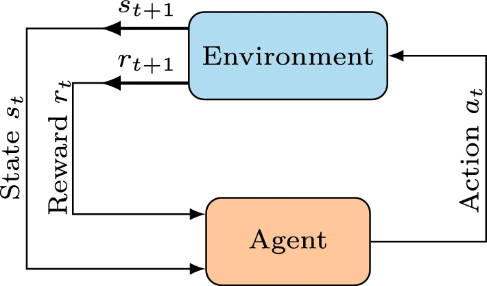
The main characters of RL are the agent and the environment.

• The environment is the world where the agent lives in and interact with. The agent sees the state, \(s\), of the environment and decide an action, \(a\), to take.
• The agent obtains a reward, \(r\), signal from the environment, a numeric value indicating how good or bad the current state is. The overall goal of the agent is to maximize its cumulated reward, return.
• A state is a complete description of the state of the world, with NO information about the world hidden from the state. An observation \(o\), possibly omitting some information, is a partial description of the state.

Deep Reinforcement Learning (RL) combines deep learning techniques with reinforcement learning to enable agents to learn optimal strategies from large volumes of complex data.

What is a policy in reinforcement learning?

A policy is a rule that used by an agent to determine its actions. A policy (\(t\) is a time step) can be described as:

• Deterministic: \(a_t = \mu(s_t)\)
• Stochastic: \(a _t \sim \pi(\cdot | s _t)\), where \(\pi\) is used instead of \(\mu\)

\(\theta\) or \(\phi \) are used when parameterized policies (learning from a neuron network, NN), we have \(\mu_{\theta}\) and \(\pi_{\theta}\) respectively.

Note: Training or using stochastic policies involves sampling actions from the policy and then calculate the log likelihoods for that action, \( \log \pi_{\theta}(a|s)\).

What is a Trajectory?

A trajectory \(\tau\) is a sequence of states and actions:

$$\tau = (s_0, a_0, s_1, a_1, …).$$

State transition at different \(t\) steps (i.e. \(s_{t}\) to \(s_{t+1}\)) can be deterministic, \(s_{t+1} = f(s_t, a_t)\), or stochastic, \(s_{t+1} \sim P(\cdot|s_t, a_t)\).

Find out the Reward function and Return

A reward function \(R\) depends on the current state of the world, the action just taken, and the next state of the world.

$$r_t = R(s_t, a_t, s_{t+1})$$

frequently simplified as current state \(r_t = R(s_t)\), or state-action pair \(r_t = R(s_t,a_t)\).

Getting reward over a trajectory yields return \(R(\tau)\):

• \(R(\tau) = \sum_{t=0}^T r_t\), for a fixed windows of steps.
• \(R(\tau) = \sum_{t=0}^{\infty} \gamma^t r_t.\) where \(\gamma \in (0,1)\), for infinite steps.

Mathematical Representation of a Reinforcement Learning Problem

In Reinforcement Learning, the main objective is to find out a policy that maximizes the expected return, regardless of the specific return measure used. This expected return is based on the agent’s actions following the chosen policy.

Before discussing expected returns, we define the probability distributions over trajectories, which are vital to calculating the expected outcomes of an agent’s actions over time – for stochastic policy \(\pi\) and transitions, the probability of a \(T\)-step trajectory is (\(\rho_0\) is the start-state distribution):

$$P(\tau|\pi) = \rho_0 (s_0) \prod_{t=0}^{T-1} P(s_{t+1} | s_t, a_t) \pi(a_t | s_t).$$

Then expected return \(J(\pi)\) is

$$J(\pi) = \int_{\tau} P(\tau|\pi) R(\tau) = \underset{\tau\sim \pi}{E}[{R(\tau)}].$$

Using \(\pi^*\) to describe the optimal policy, getting

$$\pi^* = \arg \max_{\pi} J(\pi),$$

Value functions

Value functions are central to most Reinforcement Learning algorithms. They estimate the expected return for a state or state-action pair, assuming a specific policy is followed thereafter.

• On-Policy Value Function \(V^{\pi}(s)\): Estimates the expected return starting from a state and following a given policy. $$V^{\pi}(s) = \underset{\tau \sim \pi}{E}[{R(\tau)\left| s_0 = s\right.}]$$
• On-Policy Action-Value Function \(Q^{\pi}(s, a)\): Estimates the expected return starting from a state, taking a specific action (which may not follow the policy), then following the given policy. $$Q^{\pi}(s,a) = \underset{\tau \sim \pi}{E}[{R(\tau)| s_0 = s, a_0 = a}]$$
• Optimal Value Function \(V^{*}(s)\): Estimates the expected return starting from a state and following the best possible policy. $$V^*(s) = \max_{\pi} \underset{\tau \sim \pi}{E}[{R(\tau)| s_0 = s}]$$
• Optimal Action-Value Function \(Q^{*}(s, a)\): Estimates the expected return starting from a state, taking a specific action, then following the best possible policy. $$Q^*(s,a) = \max_{\pi} \underset{\tau \sim \pi}{E}[{R(\tau)| s_0 = s, a_0 = a}]$$

Knowing the optimal action-value function \(Q^*(s,a)\), you can always figure out the best move to make in any situation by choosing the action that gives the highest \(Q^*\), which means \(a^*(s) = \arg \max*a Q^*(s,a)\), finding the action 𝑎 that maximizes \(Q^*(s, a)\).

Bellman Equations

The Bellman equations are guidelines for how to estimate the value of being in a certain state or taking a certain action in a game or decision-making process. They help us understand how good it is to be in a specific situation or to make a certain move.

The value of being in a particular state (or taking a particular action) is equal to the immediate reward you get plus the value of the next state you end up in.

• State-Value Function, \(V^{\pi}(s)\).
  • \(r(s, a)\) the reward obtained from taking action 𝑎 in state 𝑠.
  • \(V^{\pi}(s’)\) the value of next state \(s’\) following the same policy 𝜋.
  • \(\gamma\) discount factor.

$$ V^{\pi}(s) = \mathbb{E}_{a \sim \pi, s’ \sim P}[r(s,a) + \gamma V^{\pi}(s’)] $$

From Supervised Learning to Reinforcement Learning

There are a lot of machine learning tasks considered as supervised learning:

• Image Classifier: Let the machine know what the input is AND the outoput (that it is supposed to give), then train the model.
• Self-supervised Learning: Supervised learning IN REALITY, where labels can be generated automatically.
• Auto-Encoder: An unsupervised method (no human labeling), but in reality still uses labels that do NOT require humans to generate.

Reinforcement Learning, on the other hand, is quite different: You do NOT know the BEST output when you give machine an input.

What is Policy Gradient?

Imagine you’re trying to optimize a policy \(\pi_{\theta}\) ​(a strategy or set of rules that your agent follows) to maximize the expected return \(J(\pi_{\theta})\) which is essentially the total reward your agent is expected to get.

The policy \(\pi_{\theta}\) is parameterized by 𝜃, which means it depends on some parameters 𝜃 that you can adjust to improve your policy.

The policy gradient \(\nabla_{\theta} J(\pi_{\theta})\) tells you how to update your parameters 𝜃 to increase your \(J(\pi_{\theta})\) —— By following the direction of the gradient, you can make your policy better over time —— algorithms that optimize the policy this way are called policy gradient algorithms.

$$\theta_{k+1} = \theta_k + \alpha \left. \nabla_{\theta} J(\pi_{\theta}) \right|_{\theta_k}$$

Derive the analytical solution

Prepare the equations

A trajectory 𝜏, \(\tau = (s_0, a_0, …, s_{T+1})\), is a sequence of states and actions that the agent experiences from start to finish. The probability of a trajectory happening, given your policy \(\pi_{\theta}\), depends on:

$$P(\tau|\theta) = \rho_0 (s_0) \prod_{t=0}^{T} P(s_{t+1}|s_t, a_t) \pi_{\theta}(a_t |s_t).$$

Derivative of \(\log x\) with respect to \(x\) is \(1/x\). To move the derivative inside an expectation,

$$\frac{\mathrm{d} }{\mathrm{d}x}\Bigl[f\bigl(g(x)\bigl)\Bigl]=\dfrac{\mathrm{d}f}{\mathrm{d}g}\dfrac{\mathrm{d}g}{\mathrm{d}x}$$

$$ \nabla_{\theta} \log P(\tau | \theta) = \frac{1}{P(\tau | \theta)} \times \nabla_{\theta} P(\tau | \theta) $$

$$\nabla_{\theta} P(\tau | \theta) = P(\tau | \theta) \nabla_{\theta} \log P(\tau | \theta).$$

The Log-Probability of a Trajectory, \(P(\tau|\theta)\), based on \(log_{m}ab=log_{m}a+log_{m}b\),can be written as:

$$\log P(\tau|\theta) = \log \rho_0 (s_0) + \sum_{t=0}^{T} \bigg( \log P(s_{t+1}|s_t, a_t) + \log \pi_{\theta}(a_t |s_t)\bigg).$$

The environment (transition probabilities and reward function) has no internal dependence on \(\theta\). The gradients of \(\rho_0(s_0)\), \(P(s_{t+1}|s_t, a_t)\), and \(R(\tau)\) are zero. Based on \({\displaystyle \nabla (\psi +\phi )=\nabla \psi +\nabla \phi }\)

$$ \nabla_{\theta} \log P(\tau | \theta) = \cancel{\nabla_{\theta} \log \rho_0 (s_0)} + \sum_{t=0}^{T} \left( \cancel{\nabla_{\theta} \log P(s_{t+1}|s_t, a_t)} + \nabla_{\theta} \log \pi_{\theta}(a_t \mid s_t)\right) $$

$$= \sum_{t=0}^{T} \nabla_{\theta} \log \pi_{\theta}(a_t \mid s_t)$$

Derive the equations

1. Start with the definition of the gradient of the expected return: $$\nabla_{\theta} J(\pi_{\theta}) = \nabla_{\theta} \mathbb{E}_{\tau \sim \pi_{\theta}}[R(\tau)]$$
2. Express the expectation as an integral over all possible trajectories, weighted by their probabilities: $$\nabla_{\theta} J(\pi_{\theta}) = \int_{\tau} \nabla_{\theta} P(\tau|\theta) R(\tau)$$
3. Then $$\nabla_{\theta} J(\pi_{\theta}) = \int_{\tau} P(\tau|\theta) \nabla_{\theta} \log P(\tau|\theta) R(\tau)$$
4. Bring it back to an expectation form, which is easier to estimate with samples $$\nabla_{\theta} J(\pi_{\theta}) = \mathbb{E}_{\tau \sim \pi_{\theta}}[\nabla_{\theta} \log P(\tau|\theta) R(\tau)]$$

$$\nabla_{\theta} J(\pi_{\theta}) = \mathbb{E}_{\tau \sim \pi_{\theta}} \left[\sum_{t=0}^{T} \nabla_{\theta} \log \pi_{\theta}(a_t | s_t) R(\tau)\right]$$

By running policy in the environment, a set of trajectories \(\mathcal{D} = {\lbrace \tau_i \rbrace}^{N}_{i=1}\)

$$\hat{g} = \frac{1}{|\mathcal{D}|} \sum*{\tau \in \mathcal{D}} \sum*{t=0}^{T} \nabla*{\theta} \log \pi_{\theta}(a_t |s_t) R(\tau)$$