Behind Generative Models [In Progress]

Diffusion-based models, exemplified by Mid-journey, DALL-E, and Stable Diffusion, offer a unique approach to data generation by applying random noise and evolving it over time. While each model has its unique features, they all showcase the potential of diffusion-based techniques in creating high-quality, natural-looking outputs in machine learning

Background

In recent years, diffusion-based models have become a hot topic in the world of ML, offering a unique approach to generating high-quality data like images or text. Unlike traditional machine learning models, which typically operate through straightforward mapping functions, diffusion models work by applying random noise to data and evolving it over time. This results in a more organic, less predictable pattern that can generate more natural-looking images or produce more nuanced textual outputs.

Models like Mid-journey, DALL-E, and Stable Diffusion represent the cutting edge in this space. Mid-journey and Stable Diffusion are particularly focused on image generation and take advantage of an offline, open-source framework to ensure quality and accessibility. DALL-E, on the other hand, is widely celebrated for its capability to generate highly creative images based on textual prompts. While each has its own unique features and benefits, they all exemplify the power and potential of diffusion-based techniques in machine learning.

Basic Frameworks

The best-in-class image generation models typically contain the following three main components (Those three components are usually trained separately and assembled together).

Some Examples

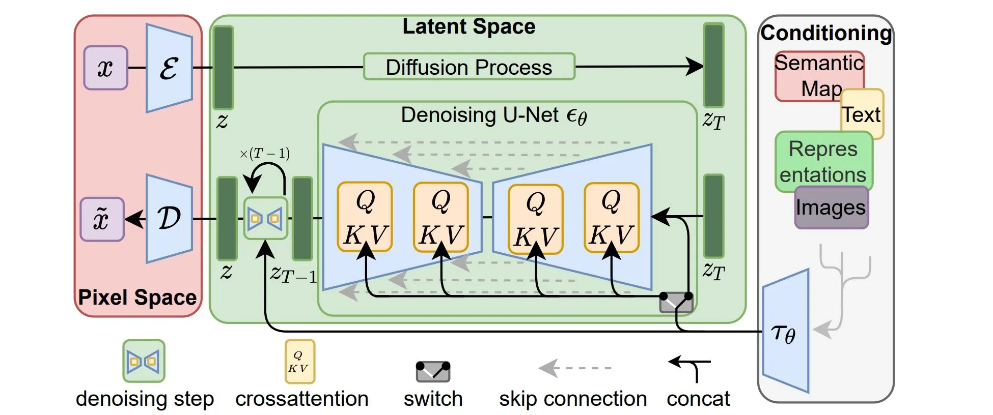
Stable Diffusion: [ Src: High-Resolution Image Synthesis with Latent Diffusion Models]

DALL-E Series: [Src1: Zero-Shot Text-to-Image Generation], [Src2: Zero-Shot Text-to-Image Generations]

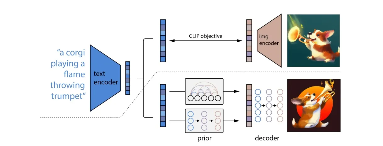
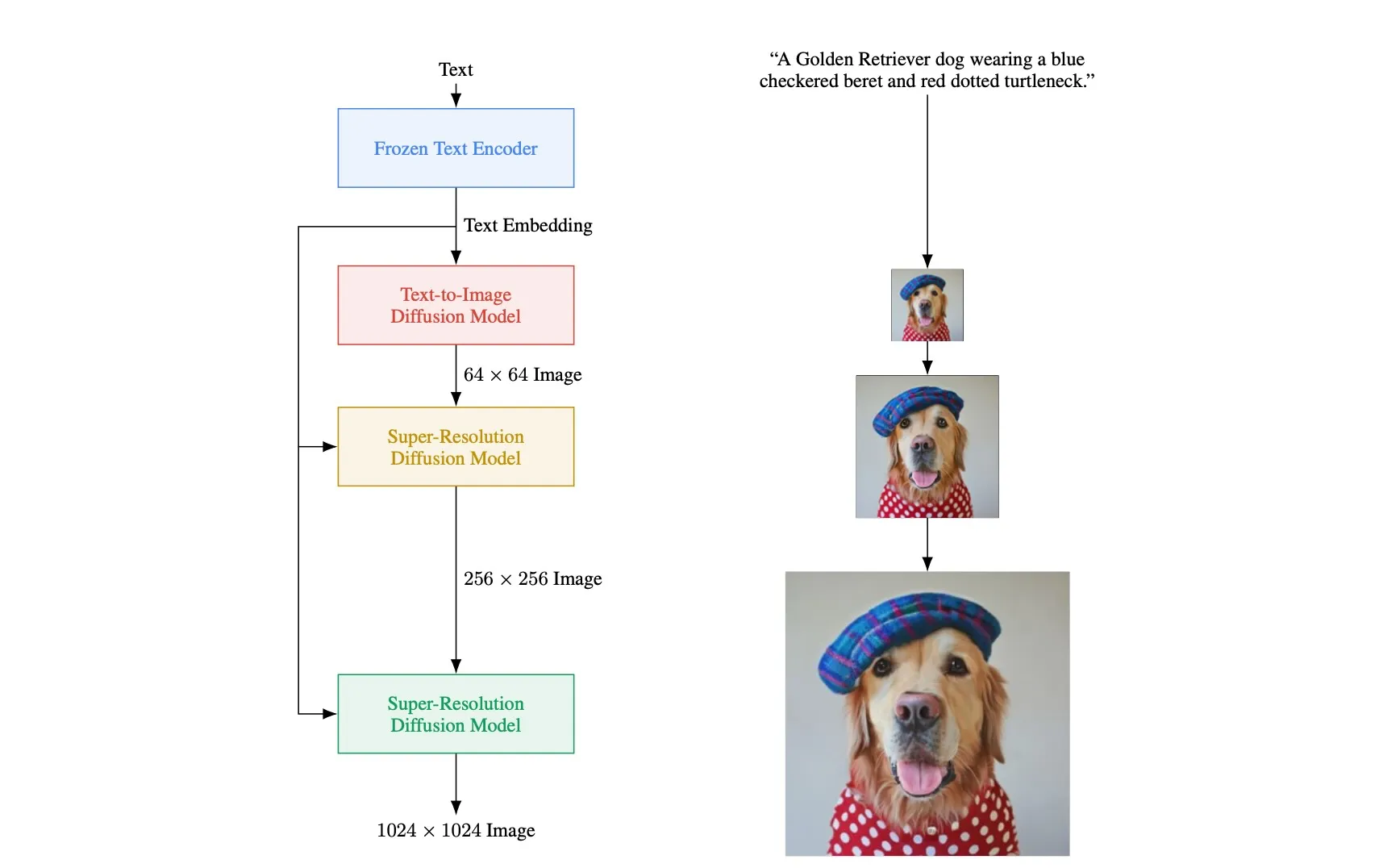
Imagen: [Src: Photorealistic Text-to-Image Diffusion Models with Deep Language Understanding]

Additional Info

Some common terms found in papers.

More about Text Encoder

FID (Fréchet inception distance) is a metric used to assess the quality of images created by a generative model. It uses a pre-trained CNN (image classification) model. You will throw images (machine-generated and real) into the CNN model to obtain their latent representations. Then you can calculate the Fréchet distance based on the assumption that both distribution are gaussian (Smaller distance means better, a lot of samples are needed).

CLIP (Contrastive Language-Image Pre-Training) utilizes 400 million image-text pairs ([link]). CLIP has an image encoder and a text encoder; they both take inputs and generate vectors (distances between vector is used to see if the image-text pair a good match).

More about Decoder

Decoder can be trained without labelled data (remember, it takes some intermediate representations, B).

1. B is a smaller image: decoder makes a bigger image.
2. B is a latent Representation: train a auto-encoder. (train an encoder-decoder pair, take the decoder)

More about Generation Model

Reminder: the Generation Model takes a vector representation of the text, and generate an (somewhat compressed) intermediate representation (or just the latent representation).

Noise is added to the latent representation during diffusion process (this is something quite unique).

1. Start with an encoder and generate some intermediate representation.
2. Add step-wise noise.
3. Train a Noise Predictor

Some Mathematics Behind

Basic Concepts

Intuitively, there are —

• Forward Process: sequentially adding noise to image till not able to see the original image.
• Reverse Process: sequentially denoising till recovering the image.

VAE vs. Diffusion Model has great resemblance. VAE uses an encoder to convert image to latent space, and use a decoder to recover image from its latent representation. The noise adding (N times) processes in the Diffusion Model can be treated as an encoder (in this case, not a NN that can be learned, it is predefined by human), and the denoising (N times) processes is like a decoder.

Denoising Diffusion Probabilistic Models

Training

• repeat
  1. $\mathbf{x_0} \sim \mathbf{q(x_0)}$ $\Lleftarrow$ sample the clean image
  2. $t \sim \mathrm{Uniform (\lbrace 1, ... ,T \rbrace)}$ $\Lleftarrow$ sample a whole number
  3. $\mathbf{\epsilon} \sim \mathcal{N}(0, \mathbf{I})$ $\Lleftarrow$ sample noise (or taget noise)
  4. Take gradient descent step on $\nabla_ {\theta} {\Vert \mathbf{\epsilon} - \mathbf{\epsilon_ {\theta}} (\sqrt{\bar{a_t}}\mathbf{x_0} + \sqrt{1 - \bar{a_t}}\mathbf{\epsilon}, t) \Vert}^2$ $\Lleftarrow$ this is rather complicated.
     1. $\sqrt{\bar{a_t}}\mathbf{x_0} + \sqrt{1 - \bar{a_t}}\mathbf{\epsilon}$ is just a noisy image, it is the weighted sum of $\mathbf{x_0}$ and $\mathbf{\epsilon}$, where $\underrightarrow{\bar{a}_1, \bar{a}_2, \dots, \bar{a}_T}$ is a set of predefined weights that gradually goes smaller.
     2. $\mathbf{\epsilon_ {\theta}}$ in $\mathbf{\epsilon_ {\theta}} (\sqrt{\bar{a_t}}\mathbf{x_0} + \sqrt{1 - \bar{a_t}}\mathbf{\epsilon}, t)$ is a noise predictor. It takes a noisy image and a number $t$
     3. The target (or ground truth) of the noise predictor is the target noise $\mathbf{\epsilon}$
• until converged.

Inference

Inference is the image generation process.

Overview:

1. $\mathbf{x_ {\mathrm{T}}} \sim \mathcal{N}(0, \mathbf{I})$ $\impliedby$ sample an all-noise image
2. for $t = T, \dots, 1$ do $\impliedby$ start of the reverse process, total $T$ times
   1. $\mathbf{z} \sim \mathcal{N}(0, \mathbf{I})$ if $t \gt 1$, else $\mathbf{z=0}$ $\impliedby$ sample another noise, $\mathbf{z}$
   2. $\mathbf{x_ {\mathrm{t-1}}} = \frac{1}{\sqrt{a_t}} ( \mathbf{x_ {\mathrm{t}}} - \frac{1-\alpha_t}{\sqrt{1-\bar{\alpha_t}}} \mathbf{\epsilon_ {\theta}} (\mathbf{x_ {\mathrm{t}}},t) ) + \sigma_t \mathbf{z}$ $\impliedby$ $\mathbf{x_ {\mathrm{t-1}}}$ is the denoised result.
      • $\mathbf{x_ {\mathrm{t}}}$ is the image generated from the previous step. The image is pure noise when $\mathbf{x_ {\mathrm{t=T}}}$
      • Inside $\mathbf{x_ {\mathrm{t}}} - \frac{1-\alpha_t}{\sqrt{1-\bar{\alpha_t}}} \mathbf{\epsilon_ {\theta}} (\mathbf{x_ {\mathrm{t}}},t)$, $\mathbf{\epsilon_ {\theta}} (\mathbf{x_ {\mathrm{t}}},t)$ is the noise output from the noise predictor.
      • Adds one more niose times a constant, $\sigma_t \mathbf{z}$
3. end for
4. return $\mathbf{x}_0$

Process:

• Prepare following two series of predefined numerical values:

$$\begin{cases} \bar{a}_1, \bar{a}_2, \dots, \bar{a}_T \\ a_1, a_2, \dots, a_T \end{cases}$$

• The noise predictor takes an image $x_t$ and $t$, yielding $\mathbf{\epsilon_ {\theta}} (\mathbf{x_ {\mathrm{t}}},t)$
  • $\mathbf{\epsilon_ {\theta}} (\mathbf{x_ {\mathrm{t}}},t)$ times $\frac{1-\alpha_t}{\sqrt{1-\bar{\alpha_t}}}$, which is used to subtract from $\mathbf{x_ {\mathrm{t}}}$
    • $a$ is step-dependent
  • multiply by a fraction $\frac{1}{\sqrt{a_t}}$
• Add noise $\mathbf{z}$ to get $\mathbf{x_ {\mathrm{t-1}}}$

So, things are getting super trippy now, we need to step back for a little bit.

Shared Goals For Generative Models

It simply looks like this:

$$z \longrightarrow \theta \longrightarrow P_ {\theta}(x) \leftrightsquigarrow P_ {\mathrm{data}}(x)$$

• Sample a vector $z$ from a known distribution
• Put $z$ into a network $\theta$ plus some condition (for txt-img models)

Maximum Likelihood Estimation

• Sample images $\lbrace x^1, x^2, \dots, x^m \rbrace$ from $P_ {\mathrm{data}}(x)$, $P_ {\mathrm{data}}(x)$ is the world of possible images (the entire process is sampling training data)
• Assume we can somehow calculate $P_ {\theta}(x^i)$, $P_ {\theta}(x^i)$ is the probability of generating any image $x^i$ from $P_ {\theta}$. (this is a difficult process, $P_ {\theta}$ is not necessarily a gaussian distribution)
• $\theta^*$ can be defined as an objective function $arg {\mathrm{max} \atop \theta} \prod_ {i=1}^m P_ {\theta}(x^i)$

Dive in

Why Maximum Likelihood is equivalent to $P_ {\theta}(x) \leftrightsquigarrow P_ {\mathrm{data}}(x)$?
Because Maximum Likelihood = Minimize KL Divergence

VAE

For VAE (Variational Autoencoder), following the process described in the previous section. Sample $z$, put in the network $\theta$ which describe the relationship $G(z)=x$

DDPM

Denoising Diffusion Probabilistic Models (DDPM)

Comparison

VAE: Maximize $log P_ {\theta}(x)$ $\implies$ Maximize $\mathrm{E}_ {q(z|x)}[log \lgroup \frac{}{} \rgroup]$

DDPM: Maximize $log P_ {\theta}(x_0)$ $\implies$ Maximize $\mathrm{E}_ {q(x_1:x_T|x_0)}[log \lgroup \frac{}{} \rgroup]$

Forward Process

$q(x_{t}|x_{t-1})=$ $\mathcal{N}(x_{t};\sqrt{1-\beta_ {t}}x_ {t-1},\beta_ {t}I)$

$q(x_{1:T}|x_{0})=\prod_{t=1}^{T}q(x_{t}|x_{t-1})$

Forward Process Reparameterization Trick

Reverse Process

$$\begin{aligned} x_{t} &= \sqrt{\alpha_{t}}x_ {t-1}+\sqrt{1-\alpha_{t}} \epsilon_ {t-1} \\ &= \sqrt{\alpha_{t}\alpha_{t-1}}x_{t-2} + \sqrt{1-\alpha_{t}\alpha_{t-1}} \bar{\epsilon}_{t-2} \\ &= \cdots \end{aligned}$$ $$x_t = \sqrt{\bar{\alpha}_ {t}} x_{0}+\sqrt{1-\bar{\alpha}_{t}}\epsilon$$

Reverse Process Variational Lower Bound

$$p_ \theta(\mathbf{x}_ {0:T}) = p(\mathbf{x}_ T) \prod^T_ {t=1} p_ \theta(\mathbf{x}_ {t-1} \vert \mathbf{x}_t)$$ $$p_\theta(\mathbf{x}_ {t-1} \vert \mathbf{x}_ t) = \mathcal{N}(\mathbf{x}_ {t-1}; \boldsymbol{\mu}_ \theta(\mathbf{x}_ t, t), \boldsymbol{\Sigma}_ \theta(\mathbf{x}_ t, t))$$

Reverse Process Variational Lower Bound Loss Function