
An in-Depth Look at Leading Computer Vision ML Models
As computer vision continues to evolve, understanding the various machine learning models driving this technology is crucial. We explore the most impactful models, highlighting key innovations.
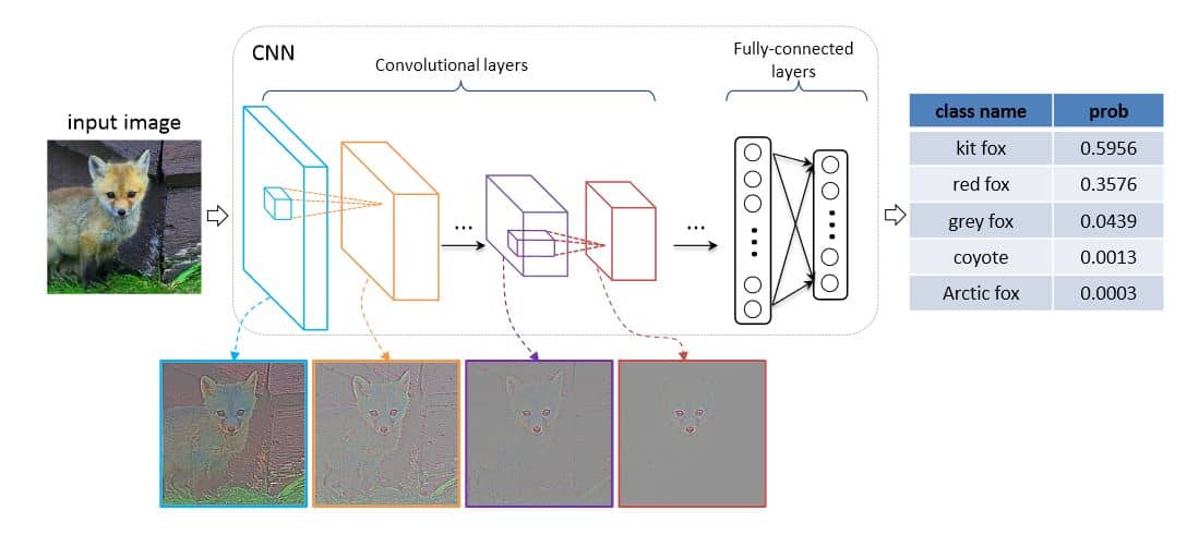
Convolutional Neural Networks (CNN)-based
CNN are used to extract features from images (and videos), employing convolutions as their primary operator.
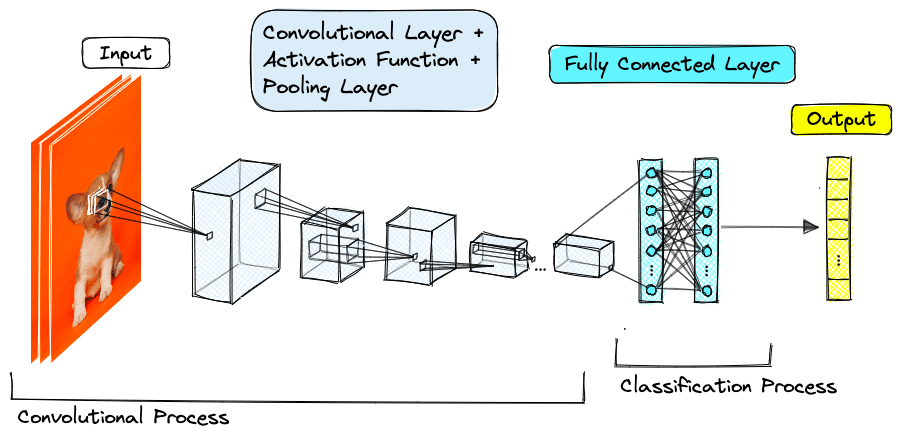
AlexNet
Designed by Alex Krizhevsky in collaboration with Ilya Sutskever and Geoffrey Hinton (University of Toronto), AlexNet (ImageNet Classification with Deep Convolutional Neural Networks, NIPS 2012) marks a breakthrough in deep learning.
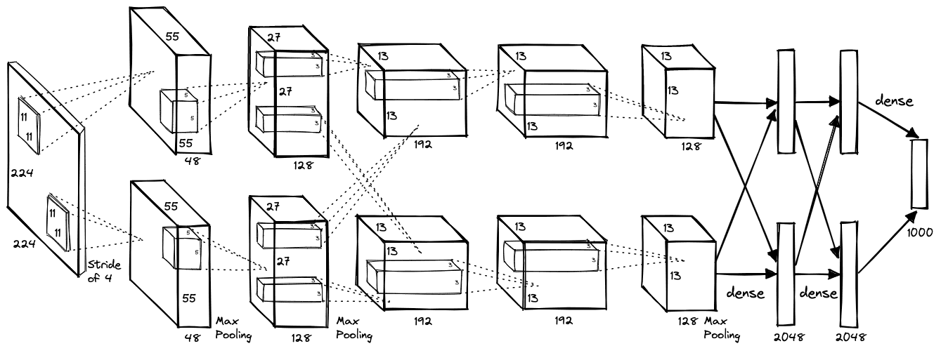
AlexNet model consisted of 8 layers: 5 conv layers followed by 3 fully-connected (FC) linear layers (Rectified Linear Unit ReLU as activation functions). A 1000-node softmax was used to produce the 1000-label classification (a probability distribution over the 1000 classes) for ImageNet.
GoogLeNet
GoogLeNet, aka Inception-v1, was for ILSVRC 2014 and CVPR 2015 Going deeper with convolutions based on the Inception architecture. An Inception Module is an image model block approximates an optimal local sparse structure in a CNN, allowing the network to extract features at multiple scales simultaneously.
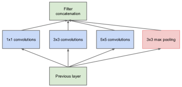
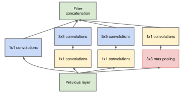
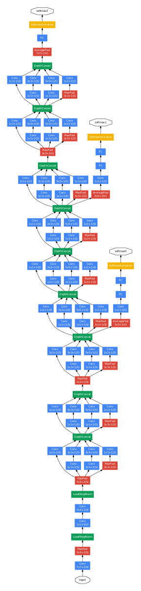
GoogLeNet has parallel convolution layers of different kernel sizes (1x1, 3x3, 5x5) as well as a max pooling layer, with the outputs concatenated before being passed to the next layer. The full GoogLeNet architecture consists of 22 layers deep.
GoogLENet v2
Or Inception-v2, comes from Rethinking the Inception Architecture for Computer Vision.
- Mini-network (3 x 3) replacing the 5 × 5 convolutions, should be around 28% reduction in calculation
(5x5 - 3x3 - 3x3)/ 5x5(more about convolution, see Simple Convolution Operation). - Authors also found an
nxnconv can be replaced by an1 x nfollowed by ann x 1(medium-sized feature maps).
Visual Geometry Group (VGG)
VGG is a convolutional neural network architecture proposed by researchers (Simonyan et al. Very Deep Convolutional Networks for Large-Scale Image Recognition, ICLR 2015) from the University of Oxford. VGG shined at the ImageNet Large Scale Visual Recognition Challenge, ILSVRC


Popular VGG-16 or VGG-19 consists of 16 or 19 convolutional layers respectively.
- Input: VGG takes in an image input size of 224×224. Creators cropped out the center 224×224 patch in each image for the ImageNet competition.
- Convolutional Layers: VGG uses 3x3 conv layers (minimal receptive field) as well as 1×1 conv filters (linear transformation).
- ReLU (from AlexNet, training time reduction than sigmoid) is also used.
- Stride (the number of pixel shifts over the input matrix) is fixed at 1 pixel, keeping the spatial resolution preserved.
- Hidden Layers: Use ReLU.
- Fully-Connected (FC) Layers: Has 3 FC layers. The first two each has 4096 channels, and the third has 1000 channels.
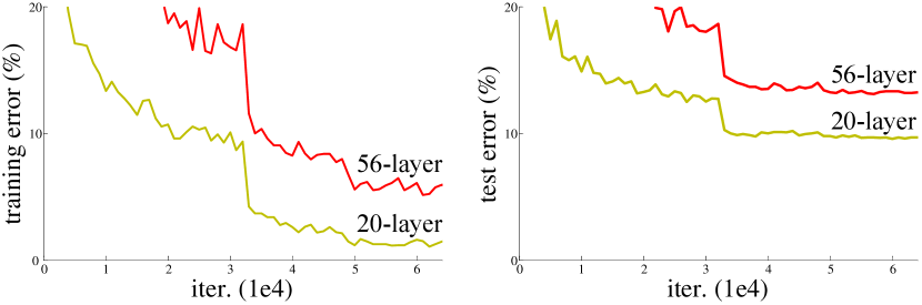
Residual Networks (ResNets)
Introduced by He et al. Deep Residual Learning for Image Recognition, CVPR 2016, ResNets were designed to address the issue where deeper network has higher training error, and thus test error (first image in the gallery below). Likely due to the gradient vanishing problem (limit for small floating number stored in each tensor) from back propagation for deeper networks.

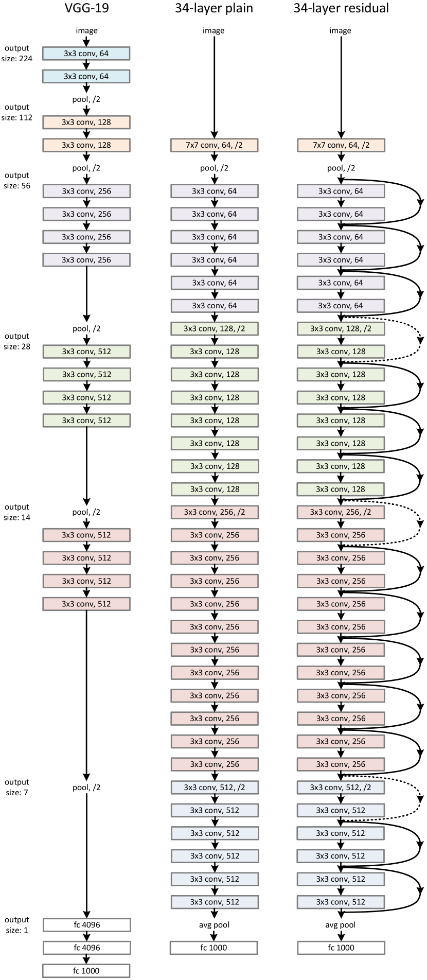
ResNets introduce a deep residual learning framework (second image in the gallery above). Shorting some of the layers for better back propagation and yields better performance.
ResNeXt
Introduced in Aggregated Residual Transformations for Deep Neural Networks. Idea: more independent heads during learning results in better performance.
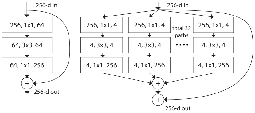
(# in channels, filter size, # out channels).Here is the performance (from Figure 5):
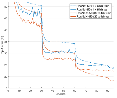
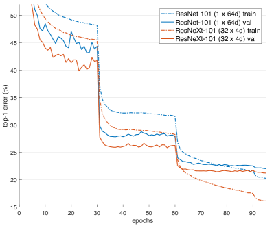
Training curves on ImageNet-1K.
Left: ResNet/ResNeXt-50 with preserved complexity ( ~4.1 billion FLOPs, ~25 million parameters);Right: ResNet/ResNeXt-101 with preserved complexity ( ~7.8 billion FLOPs, ~44 million parameters).
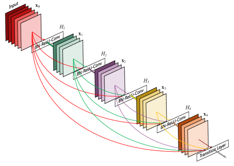
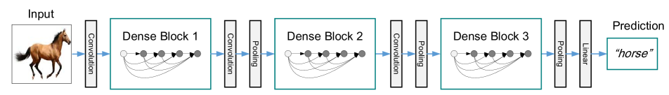
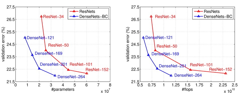
DenseNet
Introduced in Densely Connected Convolutional Networks, CVPR 2017, a DenseNet is a type of convolutional neural network uses dense connections between layers through Dense Blocks.
To ensure maximum information flow between layers in the network, we connect all layers (with matching feature-map sizes) directly with each other. To preserve the feed-forward nature, each layer obtains additional inputs from all preceding layers and passes on its own feature-maps to all subsequent layers
EfficientNet
EfficientNet EfficientNet: Rethinking Model Scaling for Convolutional Neural Networks is a CNN architecture and scaling method that uniformly scales all dimensions of depth/width/resolution using a compound coefficient (huge amount of computational power).
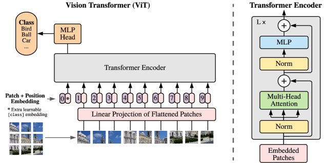
Vision Transformer (ViT)
From An Image is Worth 16x16 Words: Transformers for Image Recognition at Scale

Vision-and-Language Transformer (ViLT)
ViLT: Vision-and-Language Transformer Without Convolution or Region Supervision, ICML(International Conference on Machine Learning) 2021.
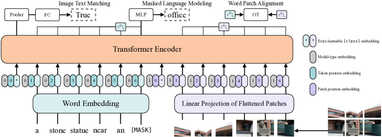
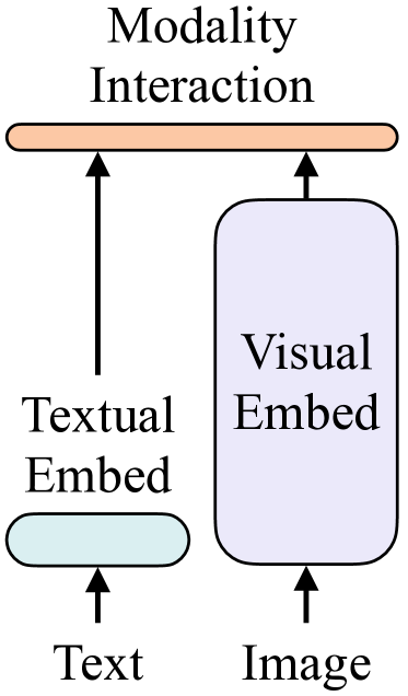

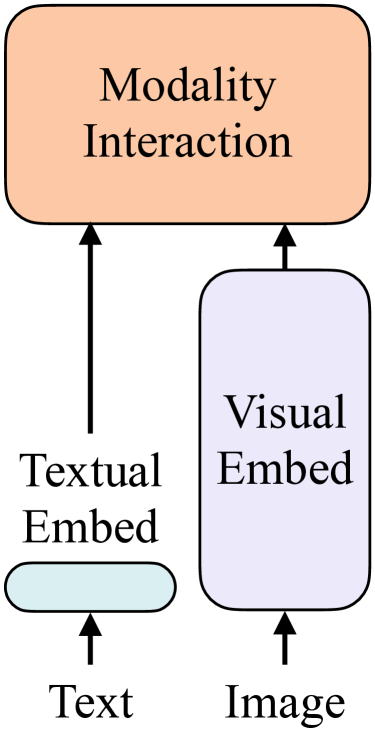
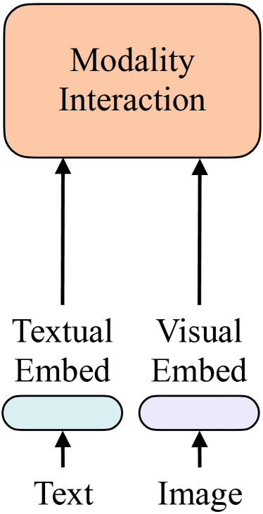
The article also mentioned 4 categories of vision-and-language models (VE, TE, and MI are short for visual embedder, textual embedder, and modality interaction, respectively.)
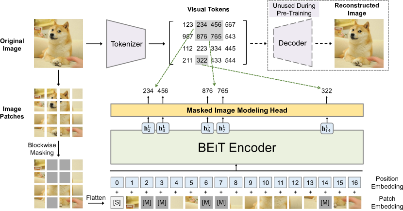
BERT Pre-Training of Image Transformers (BEiT)
BEiT: BERT Pre-Training of Image Transformers, ICLR 2022. (Bidirectional Encoder Representations from Transformers BERT, from ACL 2019, is actually a language model)
VL-BEiT: Generative Vision-Language Pretraining, is a bidirectional multimodal Transformer learned by generative pretraining.
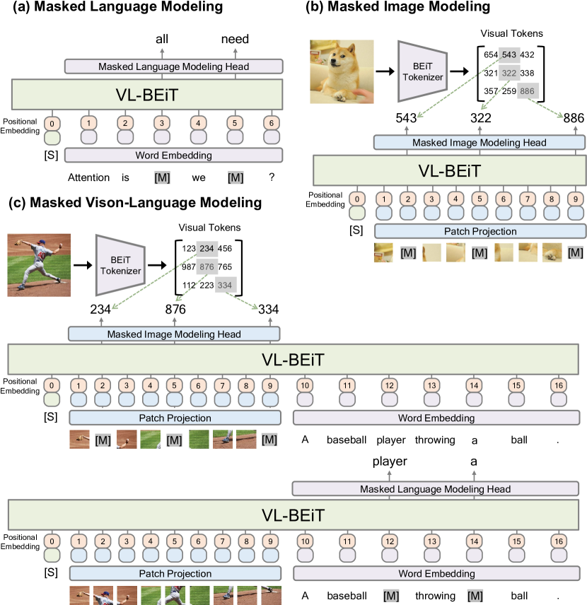
VL + BEiT.
Masked Autoencoders (MAE)
Masked Autoencoders Are Scalable Vision Learners, CVPR 2022. (strictly speaking, NOT ViT)

Contrastive Language-Image Pre-training (CLIP)
Released by OpenAI from Learning Transferable Visual Models From Natural Language Supervision. CLIP jointly trains an image encoder and a text encoder to predict the correct pairings of a batch of (image, text) training examples, and was trained from scratch on a dataset of 400 million (image, text) pairs.
Contrastive learning is a self-supervised learning approach where the model learns to differentiate between similar and dissimilar data points. The core idea is to bring similar data points (positives) closer together in the feature space while pushing dissimilar ones (negatives) apart.
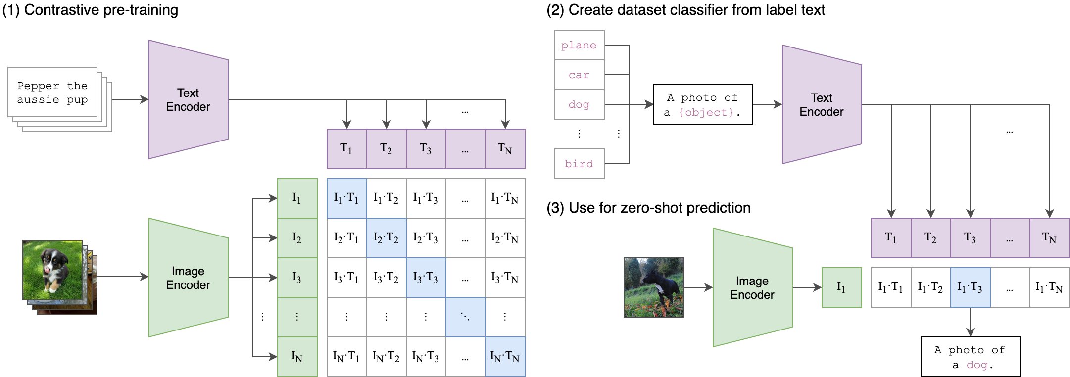
jointly trains an image encoder and a text encoder to predict the correct pairings of a batch of (image, text) training examples, while standard image models jointly train an image feature extractor and a linear classifier to predict some label. At test time the learned text encoder synthesizes a zero-shot linear classifier by embedding the names or descriptions of the target dataset’s classes.Little fun fact from the paper: The largest ResNet model, RN50x64, took 18 days to train on 592 V100 GPUs while the largest Vision Transformer took 12 days on 256 V100 GPUs
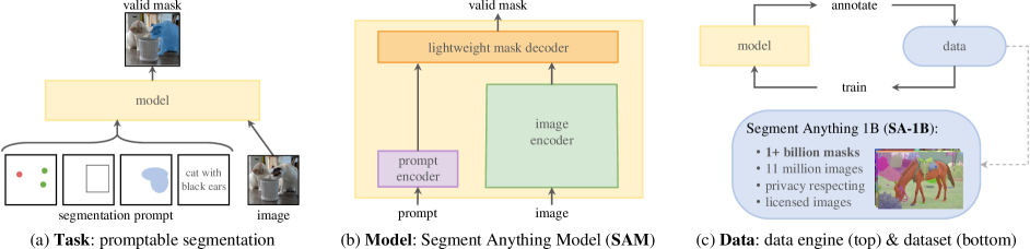
Segment Anything Model (SAM)
Segment Anything, ICCV 2023. SAM uses its own dataset with 1 billion masks on 11M licensed and privacy respecting images (SAM’s image encoder outputs 𝐶 × 𝐻 × 𝑊 image embedding, which was built upon Masked Autoencoders, MAE).
SAM2
SAM 2: Segment Anything in Images and Videos
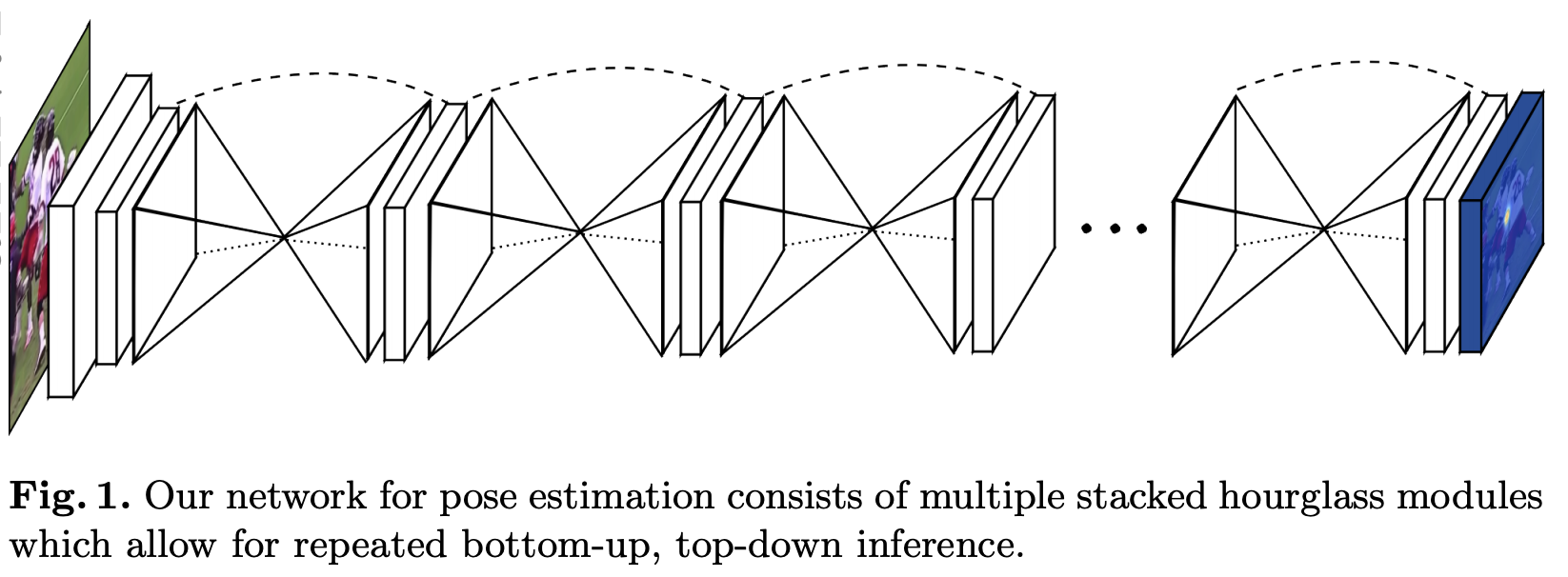
Stacked Hourglass Networks
Stacked Hourglass Networks are introduced by Newell et al. in Stacked Hourglass Networks for Human Pose Estimation
DeepPose
The DeepPose paper DeepPose: Human Pose Estimation via Deep Neural Networks, published by Google researchers at CVPR (Conference on Computer Vision and Pattern Recognition) in 2014. DeepPose was a pioneering approach at that time to human pose estimation using Deep Neural Networks (DNNs).
The core idea of the paper is to frame pose estimation as a DNN-based regression problem, predicting the coordinates of body joints
directlyfrom images (instead of treating it like a traditional classification methods)
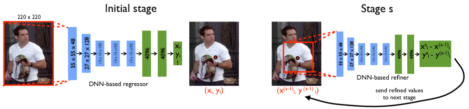
The method proposed a cascade of DNN regressors to iteratively refine pose predictions, starting with a rough estimate and improving it through successive stages.
LLaVA, Large Language and Vision Assistant
As a GPT-V alternative, researchers (Haotian Liu, Chunyuan Li , Qingyang Wu and Yong Jae Lee) used Language-only GPT-4 to generate multimodal language-image instruction-following data. By instruction tuning on such generated data, we introduce LLaVA
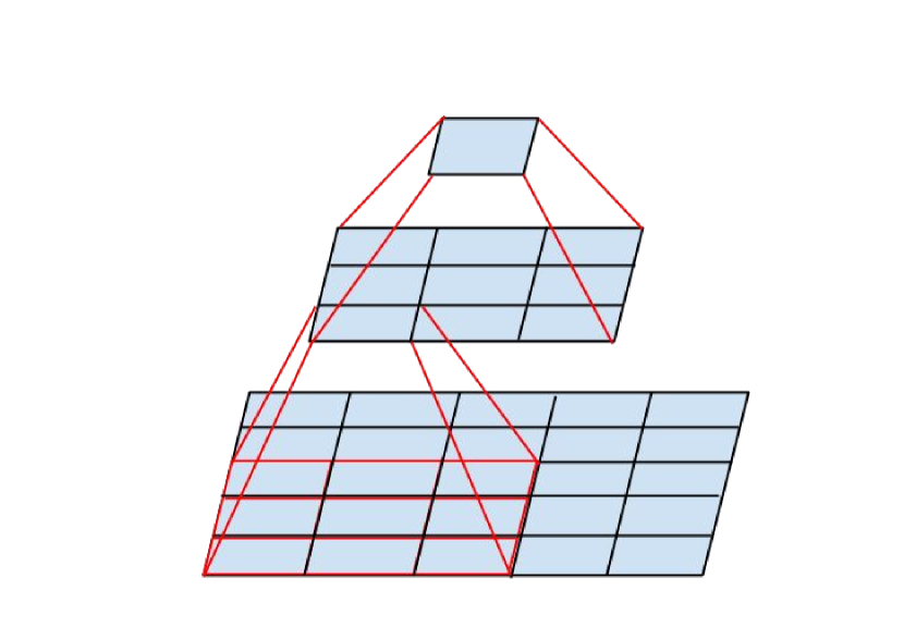
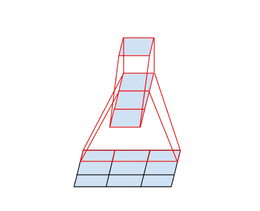
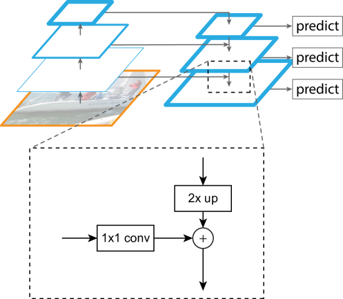
Feature Pyramid Network (FPN)

FPN is used in a lot of further development including faster R-CNN, Mask R-CNN, Single-Shot Detector (SSD), YOLO
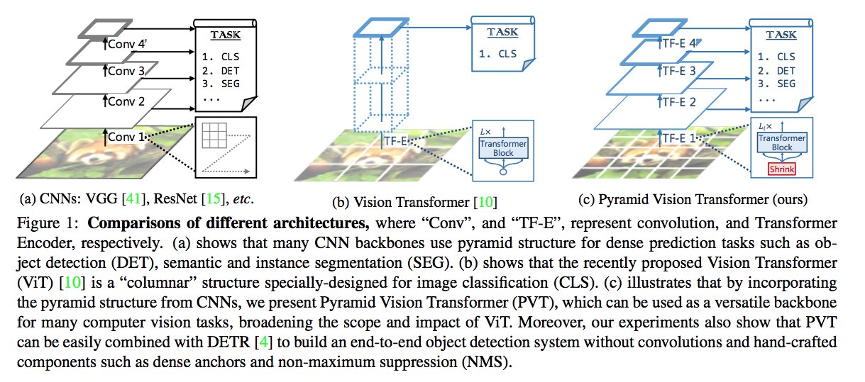
Pyramid Vision Transformer (PVT)
PVT, or Pyramid Vision Transformer, was introduced in Pyramid Vision Transformer: A Versatile Backbone for Dense Prediction without Convolutions at ICCV 2021
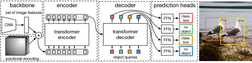
Detection Transformer(DETR)
DETR, introduced in End-to-End Object Detection with Transformers is a set-based object detector using a transformer on top of a convolutional backbone
DETR with Improved deNoising anchOr boxes (DINO)
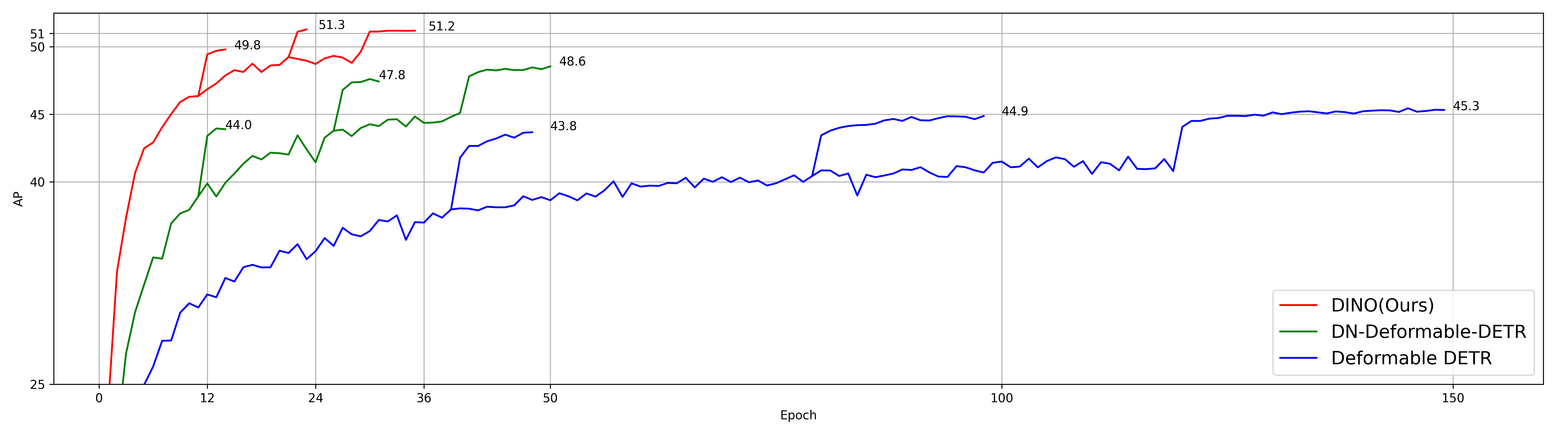
DINO is a state-of-the-art end-to-end object detector, using a contrastive way for denoising training.
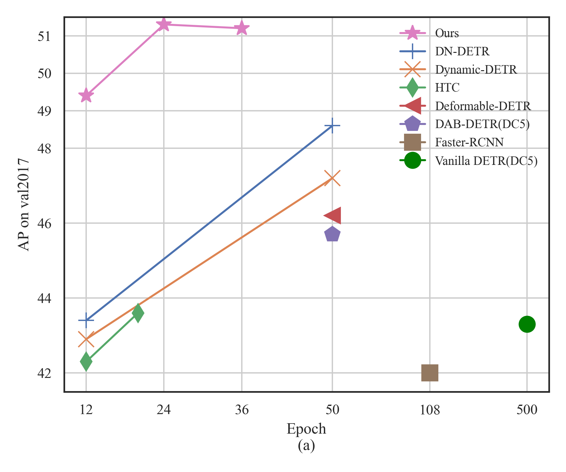
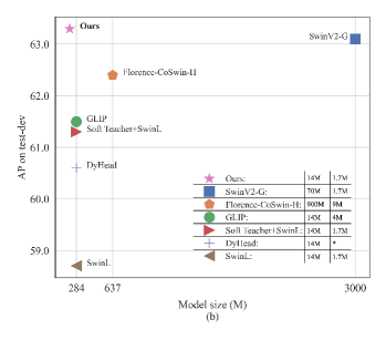
DINO achieves higher AP (Average Precision, true positives / true positives + false positives, higher the better) under less epochs while having a smaller model size, ICLR 2023.
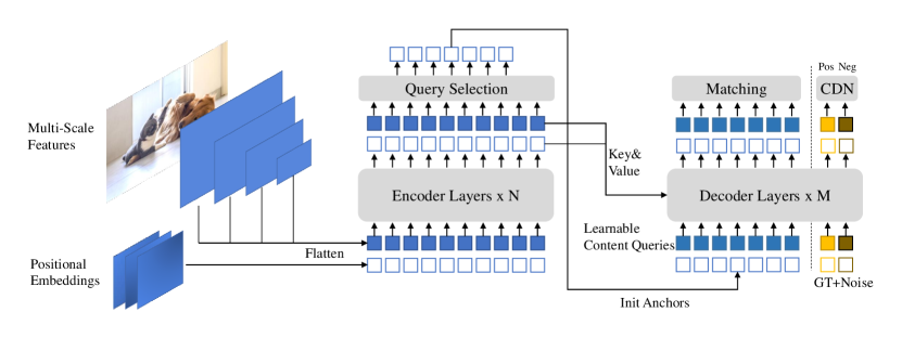
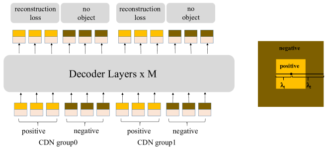
Unlike DETR, which takes the largest feature map for subsequent work, DINO takes feature maps from various scales. A positional embedding is used to help the transformer. Its Contrastive DeNoising (CDN) training section (ground true, GT + noise) is different from DETR, containing group0 and group1
- Both groups contains
positive queriesandnegative queries. - \(\lambda_{1}\) and \(\lambda_{2}\) adjusts how object stands out from the background (the size), adjusting the noise level.
CDN group0has lower noise background, hoping to learn theground truth boxes.CDN group1has higher noise, hoping to learnno object.
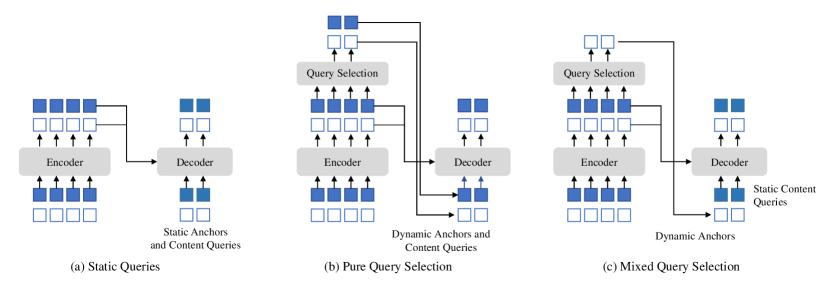

DINO uses mixed query selection. Also look forward twice (adding more connection for back-propagation), achieving great performance (DINO is around 500 epochs)